3Blue1Brown's Wordle algorithm implementation in Rust

TL;DR I just formalized 3Blue1Brown’s information theory approach to solving Wordle and implemented it in Rust for the sake of learning Rust

Wordle in one paragraph

Wordle is a single-player Mastermind variant played on five-letter English words. Each guess returns a five-symbol pattern:

• 2 / 🟩 - correct letter, correct slot
• 1 / 🟨 - letter exists elsewhere
• 0 / ⬜ - letter not in the word (or fully accounted for)

You win when the pattern is 🟩🟩🟩🟩🟩 - and you have only six guesses. A solver’s job is to choose guesses that zero-in on the secret word as fast as possible.

Algorithm

I outlined the steps of the algorithm below but you should probably watch the original video by 3Blue1Brown as that does a better job at explaining.

Step 1: Build a ‘prior’ over the answer list

Let $\mathcal{W}$ be the dictionary of 5-letter words valid in a game of Wordle, and treat the secret word as a random variable $W\in\mathcal{W}$. The probability mass function (pmf)

\[P_W(w) = Pr\set{W=w}\]

tells us how plausible each candidate is.

3Blue1Brown use a text corpus and apply a steep sigmoid that keeps the first few thousands words nearly uniform and then roll off smoothly. The corpus is sorted from most frequent to least frequent where the most frequent word has a rank $r(w)=1$.

\[\text{Weight}(w) = \displaystyle \frac{1}{1 + e^{\,\alpha\,\bigl(r(w) - 1,500\bigr)}} \qquad\qquad (\alpha \gtrsim 0.001\text{–}0.005)\] \[P_W(w) \;=\; \frac{\text{Weight}(w)} {\displaystyle\sum_{v\in{W}} \text{Weight}(v)}.\]

I used $1,500$ as where the midpoint of the sigmoid function is, but this should be adjusted based the size of the corpus. $\alpha$ is the steepness transition (higher = steeper).

Step 2: Turn a guess into a random pattern

Define the “Wordle clue function” as

$f(\mathcal{W},\mathcal{W})\rightarrow\Set{0,1,2}^5$,

Example

\[f(\text{CRANE},\text{CARER}) = (2,0,1,2,1) = 🟩 ⬜ 🟨 🟩 🟨\]

Let $X$ be the random variable to represent the 5-symbol pattern clue and $G\in\mathcal{W}$ as our guess

\[X = f(W,G)\]

where $X$ can take $3^5=\boldsymbol{243}$ values, encoded $0…242$.

Since we know the distribution of $W$ from the prior we built in step 1, we can determine the distribution of $X$ by applying transformations of random variables. Using the indicator function $\boldsymbol{1}[]$, the probability of seeing a particular pattern $x$ given $G$ is

\[P_{X\mid G}(x) = \sum_{w\in\mathcal{W}}\; \underbrace{\Pr\bigl\{W=w\bigr\}}_{=\,P_W(w)} \times \underbrace{\mathbf 1\!\bigl[f(w,G)=x\bigr]}_{1\text{ if pattern matches, else }0}\]

The equation above can be interpreted as: “add up the prior probabilities of every word that would produce pattern $\mathcal{x}$ when you guess $ G$”.

Step 3: Score a guess with entropy

For any guess $G\in\mathcal{W}$ we can compute the entropy of the pattern random variable

\[H(X\mid{G})=-\sum_{\mathcal{x}}{P_{X\mid G}(x)\log_2{P_{X\mid G}(x)}}\]

A large entropy means “this guess, on average, chops the current candidate pool into many equally‑sized chunks.” Hence the classic information‑theory policy is

\[G_{\text{entropy}} = \arg\max_{G\in\mathcal{W}}{H(X\mid{G})}\]

That policy is superb when thousands of words are still possible, but it loses its edge once the candidate set $W$ shrinks to a few dozen. At that point you also care about:

• “What’s the chance I simply hit the answer right now?”
• “If I miss, how many moves will I need afterwards?”

To balance these two effects, 3Blue1Brown defines an expected-moves function as a function of the current entropy of the candidate words set $W$.

\[S(E) (\text{units: guesses still needed})\]

where $E=log_2{|W_n|}$ is the current “bits of uncertainty.” The key approximation is

\[\mathbb{E}[\text{future moves}\mid G] = 1 + (1 - P_{W}(G))\, S\!\bigl(E - H(X\mid G)\bigr)\]

• $P_W(G)$ is the probability we hit the answer out right
• If we miss the answer, our entropy is expected to drop from $E$ to $E - H(X\mid{G})$ we then look up how many moves that entropy typically costs and weigh it the the probability $1 - P_W(G)$

Finally the best guess is

\[G_{\text{best}} = \arg\min_{G \in \mathcal{W}} \Bigl[\,(1 - P_{W}(G))\, S\!\bigl(E - H(X\mid G)\bigr)\Bigr]\]

Where does $S(E)$ come from? (Boot-strapping)

Exactly computing $S(E)$ for every real Wordle state is expensive. So it is done empirically by simulating many games with the sub-optimal guess that maximize entropy only:

1. Simulate many games that always take the max-entropy guess.
2. Record pairs (E, moves-remaining).
3. Fit / interpolate those pairs to obtain a smooth curve S(E)

Step 4: Update our Prior and repeat

After playing the best guess $G_n$, and observing the actual pattern $x_{n} = f(w_{\text{true}},G_n)$, we restrict the distribution $P_W(w)$ to only those words consistent with the pattern:

\[P_{W_{n+1}}(w) = \text{Norm}\left(P_{W_n}(w) \cdot \mathbf{1}[f(w, G_n) = x_n]\right)\]

(The $\text{Norm}$ function is just there to normalise our distribution function so that it has a sum of 1.0)

Use the new prior distribution and repeat these steps.

Rust implementation

For an implementation in Rust, see https://github.com/Nhandos/rust-wordle.

Results

Below is the result of my algorithm using this corpus with the total word list being the top 4047 most frequently used 5-letters in that corpus.

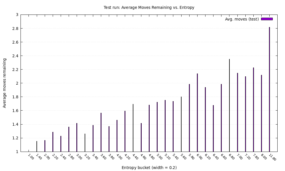
On the horizontal axis is the entropy of the candidate list and the vertical axis is how many guesses the solver still needs on average to finish. When the game begins we get around 12 bits of uncertainty and the solver typically needs 3.8 guesses on average (the y-axis shows number of guesses after the current guess, so we need to add 1).

Conclusion

I achieved what I wanted with this mini project which is to brush up on my probability and to learn a bit of rust. I got lazy towards the end and relied a bit more on generative AI than I’d like. The result shown above is probably going to be much different than 3Blue1Brown’s because they used a much larger word list.